Project Description#
The main goal of this project is to identify and predict the loan status of lenders.
To figure out whether the dataset has time series characteristic, two cross-validation methods (K-fold, TimeSplit) are also used.
In this project, RandomForest is the main model to predict and analyze the loan status.
(The Dataset for model training includes 916567 rows and 10 columns from 2007 to 2017.)
Data can be found in my
GitHub Repository
Response Variable#
- Loan_Stat -> Including 3 status, Fully Paid, Charged Off, and Default
Explanatory Variables#
Annual_Inc -> Annual incomeEmp_Length -> Employment lengthDti -> The debt-to-income ratio of the borrowerDelinq_2yrs -> The number of times the borrower had been 30+ days past due on a payment in the past 2 yearsTerm -> Borrowing termGrade -> History credit gradingInq_Last_6mths -> The borrower’s number of inquiries by creditors in the last 6 monthsPurpose -> Purpose for borrowing
Feature Engineering#
loan_stat#
- Fully_Paid -> 0
- Defult, Charged-Off` -> 1
Grade#
- A, B, C, D, E, F, D -> 1, 2, 3, 4, 5, 6, 7
Purpose#
- Debt_Consolidation -> 1
- Other -> 0
1
2
3
4
5
6
7
8
|
#getting dummies for loan_status
data_df['loan_status'] = data_df['loan_status'].str.replace('Charged Off', '1')
data_df['loan_status'] = data_df['loan_status'].str.replace('Default', '1')
data_df['loan_status'] = data_df['loan_status'].str.replace('Fully Paid', '0')

#getting dummies for purpose
data_df.loc[data_df['purpose'] != 'debt_consolidation', 'purpose'] = 0
data_df.loc[data_df['purpose'] == 'debt_consolidation', 'purpose'] = 1
|
Data Resample#
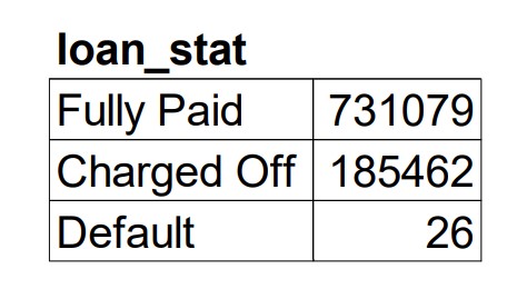
This is a very imbalance, the following plot shows that the ratio of positive data is around 20%.
I implemented the SMOTE, which is the over-sample method to increase the number of positive data.
1
2
|
# SMOTE implementation
 X_re, y_re = SMOTE(random_state=1111).fit_resample(X_train, y_train)
|
Random Forest Modeling#
Random Forest Classifier is the main model used in this project.
The following code example shows the parameters used in the RF model.
 1
 2
 3
 4
 5
 6
 7
 8
 9
10
11
12
13
14
15
16
17
18
19
20
21
22
23
24
|
def clf_original():
    #split train, test dataset
    X_train, X_test, y_train, y_test  =\
        train_test_split(X, y, test_size=0.25, shuffle = False)

    #data resample, using SMOTE
    X_re, y_re = SMOTE(random_state=1111).fit_resample(X_train, y_train)

    clf = RandomForestClassifier(n_estimators=100, max_depth=18, random_state=1111, criterion='entropy')

    clf.fit(X_re, y_re)
    train_predictions = clf.predict(X_re)
    test_predictions = clf.predict(X_test)

    cm = confusion_matrix(y_test, test_predictions)
    print(accuracy_score(y_re, train_predictions))
    print(accuracy_score(y_test, test_predictions))
    print(precision_score(y_test, test_predictions))
    print(cm)
    sorted_idx = clf.feature_importances_.argsort()
    plt.barh(X.columns[sorted_idx], clf.feature_importances_[sorted_idx])

    plot_confusion_matrix(clf, X_test, y_test)
    plt.show()
|
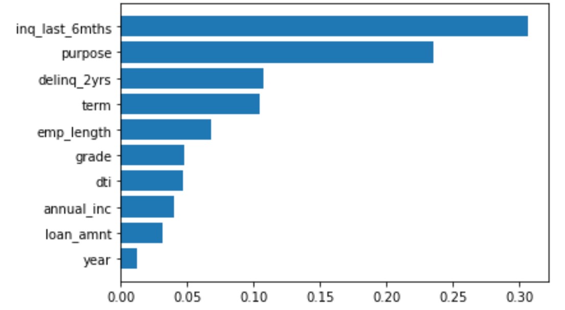 [Feature importance]
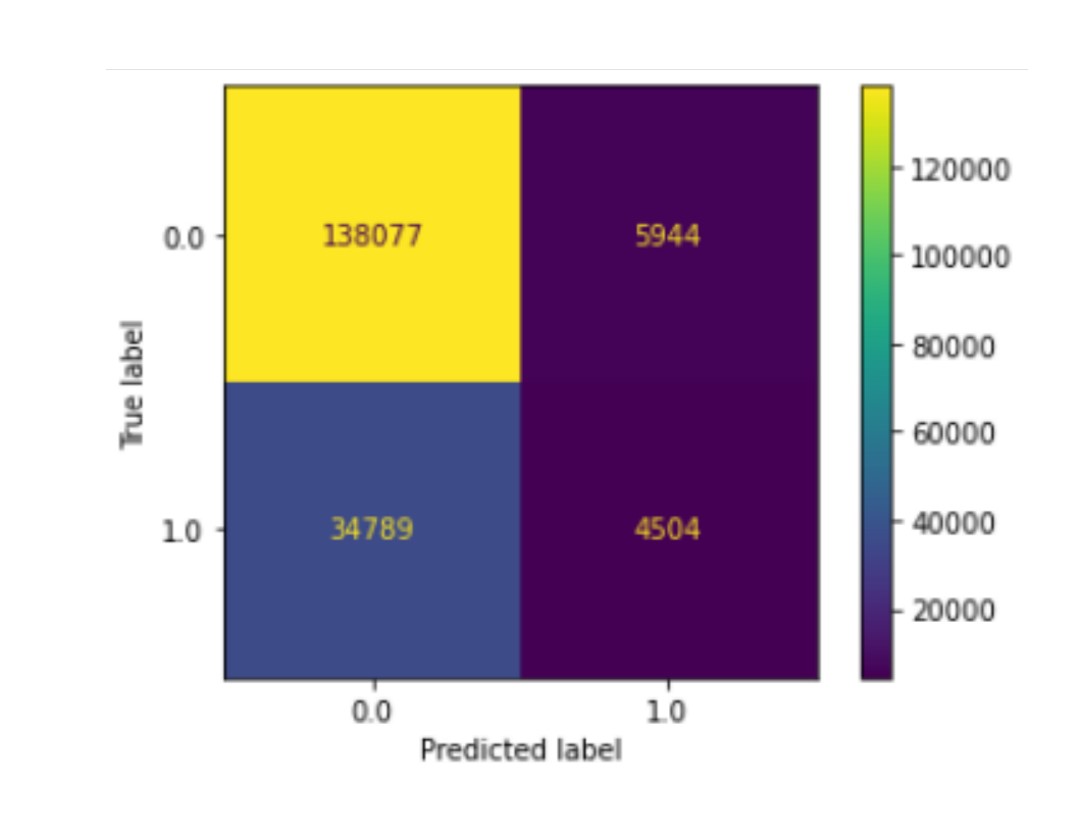 [Confusion Matrix]
Cross-Validation#
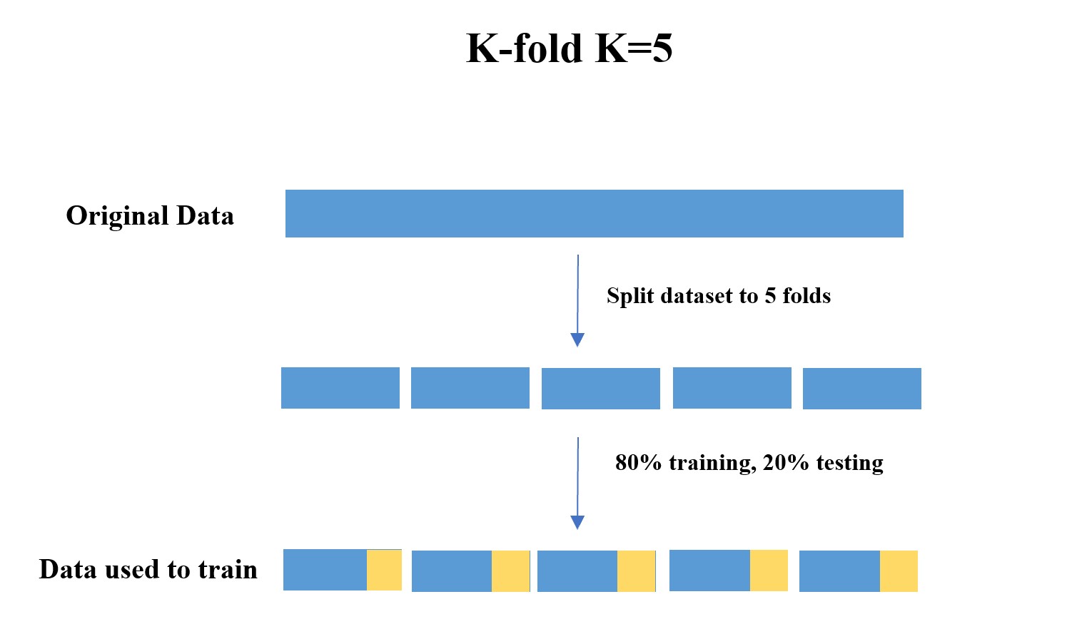
In model cross validation, I used both K-fold (K=5) and Time-Series methods to validate the RF model.
K-fold#
The dataset was first shuffle randomly then split into 5 folds.

 1
 2
 3
 4
 5
 6
 7
 8
 9
10
11
12
13
14
15
16
17
18
19
20
21
22
23
24
25
26
27
28
29
30
31
32
33
34
35
36
37
38
39
40
41
42
43
44
45
46
47
48
|
def shuffle_kfold():
    #shuffle dataset and run K-fold
    in_dic = {0:[0,146649],1:[146650,183313],2:[183314,329964],3:[329965,366628],4:[366629,513279],5:[513280,5499943],6:[549944,696594],7:[696595,733258],8:[733259,879908],9:[879909,916565]}

    avg_precison = []
    avg_recall = []
    avg_accuracy = []
    train_index = 0
    test_index = 1
    data_df_1 = data_df.sample(frac=1)
    data_df_1 = data_df_1.reset_index(drop=True)
    y_1 = data_df['loan_status']
    X_1 = data_df.loc[:, (data_df.columns!='loan_status') & (data_df.columns!='recoveries') & (data_df.columns!='total_rec_prncp') & (data_df.columns!='total_pymnt')]
    for i in range(5):
        train = in_dic[train_index]
        test = in_dic[test_index]
        X_train = X_1[train[0]:train[1]]
        X_test = X_1[test[0]:test[1]]
        y_train = y_1[train[0]:train[1]]
        y_test = y_1[test[0]:test[1]]

        X_re, y_re = SMOTE(random_state=1111).fit_resample(X_train, y_train)

        clf = RandomForestClassifier(n_estimators=100, max_depth=18, random_state=1111, criterion='entropy')

        clf.fit(X_re, y_re)
        train_predictions = clf.predict(X_re)
        test_predictions = clf.predict(X_test)

        train_accuracy = round(accuracy_score(y_re, train_predictions), 3)
        test_accuracy = round(accuracy_score(y_test, test_predictions), 3)
        avg_accuracy.append(test_accuracy )
        print(train_accuracy)
        print(test_accuracy)


        avg_precison.append(round(precision_score(y_test, test_predictions), 3))
        avg_recall.append(round(recall_score(y_test, test_predictions), 3))
        plot_confusion_matrix(clf, X_test, y_test)
        plt.show()

        train_index += 2
        test_index += 2
    avg_precision_score = sum(avg_precison) / len(avg_precison)
    avg_recall_score = sum(avg_recall) / len(avg_recall)
    print(avg_precision_score, avg_recall_score)

    return(avg_precison, avg_recall, avg_accuracy)
|
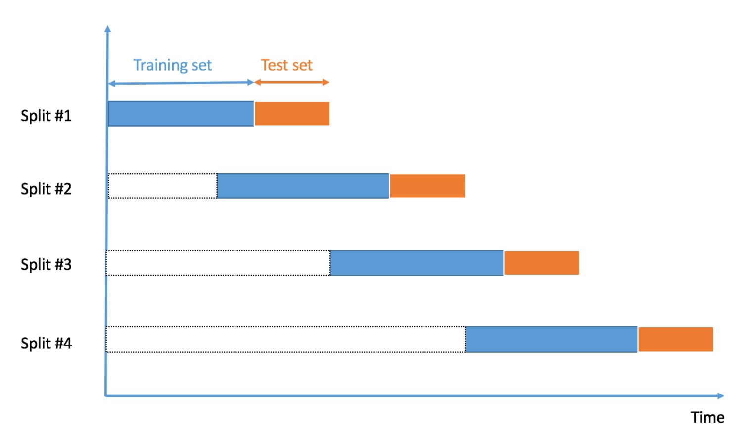
Time-Series#
The dataset was split based on the year.
Split1: 2013-2014
Split2: 2014-2015
Split3: 2015-2016
Split4: 2016-2017

 1
 2
 3
 4
 5
 6
 7
 8
 9
10
11
12
13
14
15
16
17
18
19
20
21
22
23
24
25
26
27
28
29
30
31
32
33
34
35
36
37
38
39
40
41
42
43
44
45
46
47
48
49
50
|
def time_split():
    avg_precison = []
    avg_recall = []
    avg_accuracy = []
    years_list_1 = [2013, 2014, 2015, 2016, 2017]

    for year in years_list_1:
        #filter year for train data
        train_data = data_df[data_df['year'] == year]
        #subset X, y dataset
        X_train = train_data.loc[:, (data_df.columns!='loan_status') & (data_df.columns!='recoveries') & (data_df.columns!='total_rec_prncp') & (data_df.columns!='total_pymnt') & (data_df.columns!='year')]
        y_train = train_data['loan_status']
        #count total row for training data
        row_count = y_train.count()
        #set test data size: round to interger
        test_count = int(row_count*0.2)

        X_re, y_re = SMOTE(random_state=1111).fit_resample(X_train, y_train)

        #filter year for test data
        if year<2017:
            test_data = data_df[data_df['year'] == year+1]
            #subset X, y dataset
            X_test = test_data.loc[:, (data_df.columns!='loan_status') & (data_df.columns!='recoveries') & (data_df.columns!='total_rec_prncp') & (data_df.columns!='total_pymnt') & (data_df.columns!='year')][0:test_count]
            y_test = test_data['loan_status'][0:test_count]
        else:
            break

        clf = RandomForestClassifier(n_estimators=100, max_depth=18, random_state=1111, criterion='entropy')

        clf.fit(X_re, y_re)
        train_predictions = clf.predict(X_re)
        test_predictions = clf.predict(X_test)

        train_accuracy = round(accuracy_score(y_re, train_predictions), 3)
        test_accuracy = round(accuracy_score(y_test, test_predictions), 3)
        avg_accuracy.append(test_accuracy )
        print(train_accuracy)
        print(test_accuracy)


        avg_precison.append(round(precision_score(y_test, test_predictions), 3))
        avg_recall.append(round(recall_score(y_test, test_predictions), 3))
        plot_confusion_matrix(clf, X_test, y_test)
        plt.show()
        avg_precision_score = sum(avg_precison) / len(avg_precison)
        avg_recall_score = sum(avg_recall) / len(avg_recall)
        print(avg_precision_score, avg_recall_score)

    return(avg_precison, avg_recall, avg_accuracy)
|
Result and Conclusion#
In this project, the biggest challenge is to deal with the imbalance data and come up with more creative feature engineering method.
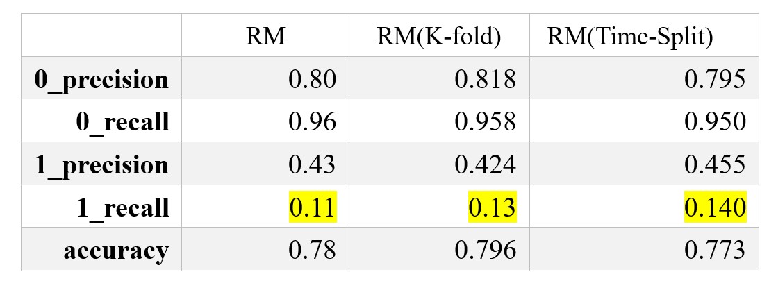
After the SMOTE was implemented, the model gains a big improvement on the prediction power on the positive data.
However, the recall rate is still low.
To improve the model performance further,hyperparameter tuning might be a good method. Since we already create the cross-validation Pipeline, the hyperparameter tuning should be easy to be added.

GitHub Repository
This is a academic project supervised by Kao, Ming-Sung from Fu Jen Catholic University. I’m very grateful to him for his enthusiastic and responsible supervision on the project.


 [Feature importance]
 [Confusion Matrix]